How to Mathematica
A practical guide for using Mathematica in problem sets
Ben Bartlett - Ruddock ‘17
2017 Ruddock Upperclassman Workshop: 24 April, 9pm
Contents:
0. Wolfram documentation
1. Formatting a notebook
Cell styles
Cell styles as folders
Math input
Suppressing output
Greek characters
Simple operator input
More complex operator input
2. Prerequisites: variables, functions, rule replacements, prefixes/suffixes, and lists
Variables
Using results from previous cells
Functions
Pattern matching in functions
Rule replacements
Prefixes and suffixes
Lists
3. Commonly-used things in Mathematica
Copy results to ![]()
Simplifying expressions with FullSimplify[]
Solving equations with Solve[]
Solving differential equations with DSolve[]
Free-form and Wolfram|Alpha input
Should I use Mathematica as a Wolfram|Alpha client?
Using free-form input in standard input cells
Working with units
Solving numerically with NSolve[] and NDSolve[]
Application: using boundary conditions
Working with vectors and matrices
Fitting functions to data
LinearModelFit[]
NonlinearModelFit[]
4. Plotting relationships and data in Mathematica
Plotting symbolic relationships with Plot[]
Plotting lists with ListPlot[]
Other common types of plots
Using Manipulate[]
0. Wolfram documentation
Mathematica has incredibly well-documented functionality. Typing any command in an input cell and hovering over the text with your mouse will bring up a dropdown menu linking to the documentation for that command. The Wolfram Language Documentation Center also has a series of excellent video tutorials that cover a lot of introductory topics to using Mathematica.
1. Formatting a notebook
Mathematica is frequently used as a scratchpad for calculations, producing messy output that needs to be inserted into a more cleanly typed problem set. However, Mathematica documents can formatted with text, images, and other media to produce well-organized content that is suitable to turn in as a problem set!
Cell styles
Using Format -> Style, (Alt + number on Windows or Cmd + number on Mac) you can change the style of a cell to make a title, subtitle, section, subsection, or text. There are a lot of options for this, but the only ones really worth remembering are (replace Alt with Cmd for Mac):
Title: Alt + 1 (Cmd + 1 on Mac)
Chapter: Alt + 2
Section: Alt + 4
Subsection: Alt + 5
Text: Alt + 7
Cell styles as folders
Mathematica also groups cells by descending section order. This allows you to collapse entire sections that you don’t need to look at. If you hover over the extended right bracket “]” spanning this section, it will turn blue. Double click it to collapse the section, and double click again to expand it again.
Try it yourself
Try changing the style of this cell to a subsection!
Math input
One of the first things that turns new people off from Mathematica is the ugly way that expressions can look when you write them down. For example,
![]()
![]()
is not the most easily readable expression. However, using the correct keyboard input, you can write this much more nicely:
![]()
If you’re just starting out using Mathematica, you might find the math palettes (Palettes -> Basic Math Assistant) useful.

Hovering over any of the buttons should display the keyboard shortcut to enter that expression in Mathematica. Learn these! They’ll save a lot of time in the future.
There is a lot of functionality here, but as usual with this guide, I’ll cover the ones most useful to know.
Suppressing output
When you evaluate a cell with Shift+enter, you’ll see an input and an output. Sometimes, for example if you’re defining a block of variables, you don’t need this output. In this case, you can suppress the output with a semicolon.
![]()
![]()
![]()
Greek characters
Any Greek character can be input into a document (in text mode or input mode) by typing esc+letter+esc. For example, esc+p+esc inputs π, esc+G+esc gives Γ, and esc+b+esc is β. This alone can easily reduce a lot of the ugliness associated with Mathematica syntax in a notebook. A few other useful similar shortcuts:
esc + ii + esc: i (imaginary number)
esc + ee + esc: e (number e)
esc + inf + esc: ∞
Simple operator input
Many common operators can be written in Mathematica using Ctrl+key (on both Windows and Mac - not Cmd). These are typically pretty easy to remember:
Ctrl + / gives a fraction: ![]()
Aside: multiplication is done by *, but can be implicitly used by simply putting a space between two variables
Ctrl + 2 gives a square root: ![]()
Ctrl + 6 gives an exponent: ![]()
Ctrl + 9 opens an inline math cell (only in text mode!): ![]()
Ctrl + - creates a subscript: ![]()
As a general rule, I wouldn’t recommend naming any of your variables with subscripts, since Mathematica has inconsistent handling of variables with subscripts in them. I always convert ![]() to “xi” in my code.
to “xi” in my code.
As usual, there are many others, but these are some of the most commonly used ones.
More complex operator input
Mathematica also has a lot of “template operators” that typeset nicely in a notebook. These are typically entered by esc + (some sensible shortcut) + t + esc. For example:
esc + intt + esc is an indefinite integral: ∫■d□
esc + dintt + esc is a definite integral: ![]()
esc + sumt + esc is a sum: ![]()
esc + prodt + esc is a product: ![]()
These can be nested too! For example,
![]()
![]()
Some operators aren’t templated, but are entered in a similar way:
esc + dd + esc is a differential symbol: d
This one is tricky - this isn’t the same as D[expr, var]. For that, you need to use the ∂ symbol
esc + pd + esc is a partial differential symbol: ∂
You can use this in place of D[expr, var]:
![]()
![]()
Try it yourself
Try entering the Ramanujan approximation of π in a new cell below.
2. Prerequisites: variables, functions, rule replacements, prefixes/suffixes, and lists
Mathematica has most data structures of other programming languages, but for use as a calculation tool for non-CS problem sets, there’s only a few that you have to know.
Variables
Variables in Mathematica can have two “types” (note that Mathematica is completely untyped, so I use this word in the loosest sense): symbolic or defined. Symbolic variables will always be blue or green in the document (they’re green if they’re used for evaluating something, like in plotting), while defined variables, which can be either expressions of symbolic variables or numbers, are black. You can clear defined variables using Clear[var1, var2, var3...]
Using results from previous cells
You can use previously computed results either by storing them to a variable (usually preferred) or by using the % operator, which gets the last Out[] result computed in the notebook. Note: this is the last value computed, not necessarily the previous cell!
![]()
![]()
![]()
![]()
Using %%...% gets the (number of %’s) previous cell:
![]()
![]()
![]()
![]()
And using %n or Out[n] uses the n’th output:
![]()
![]()
Functions
Built-in Mathematica functions always start with a capital character. You can also define your own functions. Mathematica admits two types of “functions”. You can define variables to be “expressions” of symbolic variables with an = symbol, or you can define formal functions that use lazy evaluation using a transformation rule on a symbol (x_, for example), and a := symbol. For example:
![]()
![]()
![]()
Pattern matching in functions
You can use existing symbols to create inferred functional patterns. For example, if I wanted to define the tensor product of two vectors (typically denoted by KroneckerProduct[v1, v2]) using the standard ⊗ notation, I could use:
![]()
![]()
![]()
Rule replacements
Mathematica is a functionally-styled programming language, and has nice rule replacements. You can replace any symbol in an expression with another expression by using a rule replacement: “/.”
![]()
![]()
![]()
![]()
Prefixes and suffixes
These aren’t terribly important, but can save you time typing and make your input look more nicely formatted. You can add a prefix or suffix to any function by using the @ and // operators, respectively. These work with any function that takes only a single argument. For example:
![]()
![]()
![]()
![]()
![]()
![]()
Lists
Lists in Mathematica are simply collections of items (that don’t have to be of the same type) and are handled similarly to Python, with a few exceptions. They are entered using curly braces: {item1, item2, item3}.
![]()
Lists are 1-indexed (important!) and can be sliced with the [[ ;; ]] operators:
![]()
![]()
![]()
![]()
![]()
![]()
You can also generate lists with a Table[] function:
![]()
![]()
![]()
![]()
There are a lot of other list manipulation functions available in the documentation.
3. Commonly-used things in Mathematica
Mathematica can be an indispensable tool for use in your problem sets. Although the language has basically everything you could ever think of built in as dedicated functions, you’ll find yourself using a handful of functions fairly often. I’ll cover these below.
Copy results to ![]()
If you use ![]() to type up your problem sets, you can copy results from Mathematica output by selecting the desired output and selecting “Copy As ->
to type up your problem sets, you can copy results from Mathematica output by selecting the desired output and selecting “Copy As -> ![]() ".
".
Simplifying expressions with FullSimplify[]
There’s a lot of built-in simplification functions and expression manipulation functions (Expand[], Factor[], Together[], etc.), but the go-to function is always FullSimplify, which will get you the result you want about 80% of the time, anecdotally.
![]()
![]()
![]()
![]()
You can also use FullSimplify to verify solutions satisfy an equation
![]()
![]()
![]()
![]()
Solving equations with Solve[]
Solve[] lets you solve an algebraic equation or system of equations for possible solutions. Note that when using Solve[] (or any other similar function, like NSolve, DSolve, etc), you need to use the test equality operator == rather than the assignment operator =, just like you would in Python. Solve[] gives a list of rule replacements, not a list of solutions, so if you want to assign something to a value from Solve, you need to destructure the list (First[] and Last[] are frequently helpful here) and apply the corresponding rule replacement to isolate the variable.
![]()
![]()
![]()
![]()
![]()
![]()
![]()
![]()
![]()
![]()
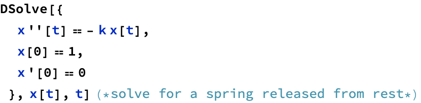
Solving differential equations with DSolve[]
DSolve[] works very similarly to Solve[], except that it requires initial conditions in some cases. (As of Mathematica 10, there’s also a handy function to retrieve the solutions, rather than rule replacements, from DSolve, which is the wrapper function DSolveValue[].) When typing the equations, use ‘ to denote derivatives with respect to the independent variable.
![]()
![]()
![]()
![]()
![]()
Free-form and Wolfram|Alpha input
As of Mathematica 8, you can use “free-form input” to express what you want to do in natural language. Mathematica is generally pretty good at figuring out what you’re trying to do. It also allows an extension of this: free-form Wolfram|Alpha input.
To use free-form input, press “=” in any blank code cell to switch it to free-form mode. Pressing “=” again will switch it to Wolfram|Alpha input, and pressing “=” a third time cycles it back to normal input. The use of both input styles is shown below.
![]()
In[50]:=
integrate 5x^2 from x=2 to x=5
Should I use Mathematica as a Wolfram|Alpha client?
Probably not. Mathematica can be a challenging platform to learn, and it’s alright to use Wolfram|Alpha if you don’t know how to do something, but, in my experience, Wolfram|Alpha stops being useful for physics problem sets around sophomore year. There are a tremendous number of things Mathematica can do that Wolfram|Alpha simply can’t, and you will eventually see some of those things appearing in your problem sets.
Using free-form input in standard input cells
If you press Ctrl+“=” (on both Windows and Mac), you can enter a small portion of free-form input in a portion of a standard input cell. This is extraordinarily useful when working with units! (See later in this section for working with units.) For example,

![]()
Working with units
Mathematica has an excellent and robust units system. The formal command for using units is Quantity[]:
![]()
![]()
However, the easiest way to input units, and the way I almost always use, is with free-form input using Ctrl+“=”.
![]()
![]()
Using UnitConvert[], you can convert some arbitrary expression into any equivalent set of units. Or, more frequently, you’ll just want to convert it to SI:
![]()
![]()
![]()
![]()
You can also look up a huge amount of quantitative data using free form input! For example, using “gravitational constant”, “earth mass”, and “earth radius” in free-form input boxes, I can calculate the surface acceleration of the Earth:
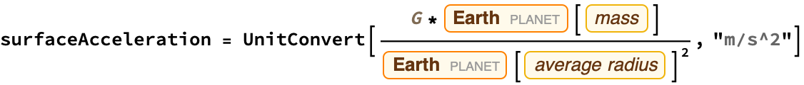
![]()
Solving numerically with NSolve[] and NDSolve[]
As you probably know, many differential equations are not analytically solvable (and some algebraic equations are gross), so you can use Mathematica’s built-in numerical solvers to work with these types of equations. NSolve[] works almost exactly the same as Solve[]:
![]()
![]()
When using NDSolve[], you’ll get a numerical “InterpolatingFunction” as an output:
![]()
![]()
You can use this InterpolatingFunction exactly as you would a regular function:
![]()
Application: using boundary conditions
As of Mathematica 10, it allows you to input Neumann and Dirichlet boundary conditions when numerically solving differential equations! For example, this is the solution to the potential throughout a metal plate with current passing through it via wires attached at the midpoints of the short end:
Working with vectors and matrices
Matrices in Mathematica work the same way they do in Python, except with the changes you’ve already seen for how vectors work. You can make matrices as lists of lists:
![]()
There are lots of matrix operations you can do. For example, you can transpose a matrix and display it like it would be written on paper:
![]()
![]()
You can find the eigenvectors and eigenvalues of a matrix:
![]()
![]()
You can multiply matrices and vectors together with the “.” operator:
![]()
![]()
And you can retrieve the magnitude of a vector with Norm[]:
![]()
![]()
Lots of vector calculus operations will require you to work with vectors and matrices. For example, you can take the curl of a vector field in Mathematica:
![]()
![]()
You can also do this using esc+delx+ esc to make a nice pretty template:
![]()
![]()
Mathematica also allows for very easy coordinate changes. For example, you can take the curl of something in spherical coordinates:
![]()
![]()
Fitting functions to data
Although it isn’t the program’s primary purpose, Mathematica includes a lot of statistical manipulation functions. The most commonly used of these, in my experience, is the fitting functions LinearModelFit[] and NonLinearModelFit[]. Let’s try these out:
LinearModelFit[]
![]()
![]()
![]()
![]()
![]()
We can do more complex stuff with LienarModelFit[] too, like fitting data to multiple variables:
![]()
![]()
Or fitting data to functions of variables:
![]()
![]()
NonlinearModelFit[]
Sometimes you get data that depends on some functional forms of variables. For example, if we considered “noisy” radioactive decay:
You can fit this type of data to a model using NonlinearModelFit[] and specifying the desired form of the data along with the constants to solve for. For example, in this case, we know decay rate follows ![]() , so we can do:
, so we can do:
![]()
![]()
![]()
4. Plotting relationships and data in Mathematica
Plotting symbolic relationships with Plot[]
Mathematica’s plotting functionality is the easiest to use and most robust of any library I’ve come across. Plot[] is your bread-and-butter function here, and can be used to plot arbitrary symbolic relationships:
![]()
You can also use Plot[] with lazily-defined (:=) functions:
You can add legends with the option PlotLegends, axes labels with AxesLabel, and many other possibilities available in the documentation.
![]()
Plotting lists with ListPlot[]
ListPlot[] works similarly to plot, but on lists of data rather than functional relationships. For example:
![]()
Other common types of plots
Other useful plot functions include ContourPlot[], Plot3D[], ListContourPlot[], and ListPlot3D[]. Extensive documentation is available for these functions, so I’ll just demonstrate one of each:
![]()
![]()
![]()
![]()
Using Manipulate[]
This is one of my favorite features of Mathematica: using Manipulate[], you can create interactive plots that allow you to explore the behavior of something as a function of some input variable(s). For example:
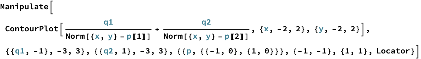
![]()
You can do a lot of really cool things with this. For example, here’s a plot of the equipotential lines from two charge sources: (you can adjust the sliders to adjust the magnitude of the charges and drag the positions of the charges around in the plot)
And here’s a manipulable solution to the Rossler attractor (a set of chaotic differential equations) displaying the behavior of all component coordinates: